Implementing cross-validation
How do we validate models?
Although our basic Machine Learning implementation is now working, it is quite limited by the fact that we have to guess the three parameters of the model. Because of this we have no way of knowing whether our choice in parameters is correct, or whether the model we have created is a particularly good model. In fact, the trained model does not really have a built in mechanism for identifying whether it is the right model or not. It is simply an optimization algorithm which provides the mathematically best fit for a function as defined through its parameters for a given set of data. Although in this simple case we might be able to tell visually whether the model is a good fit (by how well the interpolated price matches that of the points), this kind of visual analysis becomes increasingly harder, if not impossible, when approaching higher dimensional problems.
The problem becomes even more apparent when dealing with real world data, which always contains some level of error and noise. Although Machine Learning models are capable of modeling any level of complexity, there is a point at which the model stops modeling the underlying system generating the data, and starts to model the noise that is particular to the training data set. If you set all the parameters in such a way that maximum variance is produced, it is actually possible for any algorithm to perfectly model every single data point. But since the data is probably noisy, it is unlikely that such a model would scale well to other data that is part of the same system but was not considered during training. This problem is known as overfitting, and the parameters of the model are your tools to constrain the model to avoid this overfitting from happening. However, if you cannot visualize the data set and the model, how can you tell the point at which a model becomes too complex, and starts to model the noise in the training set rather than the underlying system which created it?
The process of choosing an appropriate model and tuning its parameters for a particular data set is known as validation, and it is one of the most fundamental issues in Machine Learning. Although this issue is difficult and there is no single answer for how to perform such validation, the practice of Machine Learning has produced several heuristics or common ‘best practice’ methods for how to address it, based on techniques which have generated good results in the past. One of the most popular methods is called cross-validation, which involves training the model on only a portion of the data, while keeping the rest of the data hidden from the training algorithm. Once the model is trained, its performance is then judged based on how well it describes the hidden (or validation) data set. Since this data set was not considered in the training, its noise could not have influenced the model. It is thus considered a good measure of how well the model is representing the actual system that generated both sets of data. To achieve the ‘best’ model, a researcher typically trains many models, and then picks the one that has the best performance in the validation set. For a good discussion of the overfitting problem, how it relates to the bias-variance tradeoff, and how it can be addressed through cross-validation, you can read through this helpful article.
Setting up cross-validation
Scikit-learn offers a number of helpful tools for performing cross-validation, which are described in this article. You are encouraged to explore these tools for more advanced applications of supervised learning. However, for the purposes of this demo, we will implement cross-validation manually so you can see how it works and its basic principles. We will do this again on the server side, by augmenting some of the code we wrote in the previous tutorial. Switch to the 03-validation branch in the ‘week-6’ repository, and open the app.py file in a text editor. This file has all the current code for our Web Stack server, including the basic Machine Learning application we wrote last time.
Find the lines that read:
X = np.asarray(featureData, dtype='float')
y = np.asarray(targetData, dtype='float')
These are the lines that converted the feature and target data sets into numpy arrays. In the previous example, we were using the whole data set to train the model. Now we want to split both of these arrays into two data sets: one that we will use to train the models, and one we will reserve for validating them. First, let’s determine how much of the data will remain for training, and how much will be set aside for validation. A typical approach is to use around 70% for training, and to keep around 30% for validation. Although these values depend on your particular application, including the amount of data you have and the type of model you’re training, a 70/30 split is typically a good place to start. On the following lines, type:
breakpoint = int(numListings * .7)

print "length of dataset: " + str(numListings)
print "length of training set: " + str(breakpoint)
print "length of validation set: " + str(numListings-breakpoint)
This code establishes the split between the two data sets by calculating the size of the training set as 70% of the length of the total data set. We then print out a few messages to give us feedback about the total number of data points we are working with, and the relative size of the training and validation sets. For the purposes of this exercise I suggest limiting your map scope so you are getting around 2,000 data points. If your query is returning many more points, be prepared that training the model could take a long time. This becomes a particular issue with cross-validation, since we will now be training a range of models before picking the one with the best performance.
Next, let’s split both the X and y data sets into training and validation sets based on the breakpoint we established earlier:
X_train = X[:breakpoint]
X_val = X[breakpoint:]

y_train = y[:breakpoint]
y_val = y[breakpoint:]
Here we are using the ‘:’ to subset a list. This basically takes data from a list starting with the value to the left of the ‘:’, and ending with the value to the right of it. If you leave out either value, Python assumes that you want to start at the beginning of the list or end at the end of it respectively. Now that we have split our lists into training and validation sets, we need to change our code so that the training is only happening based on the X_train data set instead of the whole X set. The next two lines should be where the training data is scaled to mean 0, variance 1. Change these lines to read:
scaler = preprocessing.StandardScaler().fit(X_train)
X_train_scaled = scaler.transform(X_train)
Training the models
The next part of the code creates and trains the SVR model. This time, instead of training a single model, we want to create a nested loop structure which will iterate over a range of values for each of the three parameters, and create a separate model for each combination of parameters. Since we will no longer be training the model based on arbitrary parameters, you can delete the lines that read:
C = 10000
e = 10
g = .01

model = svm.SVR(C=C, epsilon=e, gamma=g, kernel='rbf', cache_size=2000)
model.fit(X_scaled, y)
Now in their place, add the following code:
mse_min = 10000000000000000000000

for C in [.01, 1, 100, 10000, 1000000]:
	for e in [.01, 1, 100, 10000, 1000000]:
			for g in [.01, 1, 100, 10000, 1000000]:

				q.put("training model: C[" + str(C) + "], e[" + str(e) + "], g[" + str(g) + "]")

				model = svm.SVR(C=C, epsilon=e, gamma=g, kernel='rbf', cache_size=2000)
				model.fit(X_train_scaled, y_train)

				y_val_p = [model.predict(i) for i in X_val]

				mse = 0
				for i in range(len(y_val_p)):
					mse += (y_val_p[i] - y_val[i]) ** 2
				mse /= len(y_val_p)

				if mse < mse_min:
					mse_min = mse
					model_best = model
					C_best = C
					e_best = e
					g_best = g
The first line of code creates a variable called mse_min which we will use to keep track of the model with the smallest error. ‘MSE’ stands for Mean Squared Error, which is a very typical way of calculating the error in a model. To calculate it we first find the difference between the actual value of each validation point, and the predicted value generated by the model. We then square this value to get rid of any negative values and penalize higher errors. Finally, we add all of these values together and divide by the number of values to get their average or mean value. We initialize the mse_min variable with a very large number, so every time we come across a model with a smaller error value we will know that this is the best performing model so far.
Next, we will create a nested loop structure to iterate over a range of values for each parameter of the SVR model. We will set up a separate loop for the C, epsilon, and gamma parameters. For each parameter we will define a discrete set of values that we want to use to generate the models. In this case, we will test four values for each of the parameters, which will generate 4 x 4 x 4 = 64 models total. Although the choice of these four values is somewhat arbitrary, it is recommended to initially pick values that cover a very wide range at exponential spacing. In this case each successive value is 100 times as large as the previous one. Once you determine which values create the best performing model for a particular set of data, you can adjust these parameters for further testing. If the value of the best performing model is at the low or high extreme of the range, you can add additional values at that extreme to explore further. If the value of the best performing model is within the range, you can introduce new values around the best performing value to fine tune the model even further.
Within this set of nested loops, we write code to train one model for each combination of parameters, make predictions on the values in the validation set, and compare those predictions to the actual values to derive the MSE of each model. We then compare this MSE to the current lowest MSE value, and if the new value is lower we store the model in a new variable. By the end of this nested loop, this variable will contain the best performing model, which we will use to predict the values in the analysis grid.
Before training the actual models, we push a message with the current parameter settings to the queue so that the user knows which model is being trained. This kind of detailed messaging becomes very important as we start to develop more involved types of analyses which might have a series of steps and take much longer to execute. This way, even if the analysis takes a long time, the user will get some feedback on the process and won’t wonder whether the server has frozen or crashed. Here the SSE technology we developed for asynchronous messaging becomes crucial, since these messages can be passed and visualized by the client at the same time that the analysis is running on the server.
Following this message, we have the same two lines of code for specifying and fitting the model as before, except this time we use only the X_train_scaled and y_train data sets to train the model. Cross-validation only works if the validation data set is never seen by the training algorithm, so make sure to keep these data sets separate. On the next line, we use a loop to iterate over all the entries in the X_val array (which is storing all the features in the validation data set), and use the current model to predict their values. This single line loop is a shorthand in Python which allows you to write compact loops that generate a new list by applying a single operation to every entry in a list. In this example, this loop:
y_val_p = [model.predict(i) for i in X_val]
would be equivalent to this loop:
y_val_p = []
for i in X_val:
	y_val_p.append(model.predict(i))
in the typical syntax.
On the next four lines, we calculate the MSE of the current model’s prediction on the validation set. To do this we initialize a new variable called mse at 0. We then iterate over each predicted value, compare it to the actual value (stored in the y_val array), and square the result. We add each of these values to the mse variable, which gives us the sum of all the errors. Finally, we divide this sum by the total number of predictions to get the MSE of the current model. We then compare this MSE value to the current minimum error value. If the error is smaller, we take this model as the best performing model so far. We set the minimum MSE value to the current MSE value, and store the current model in a new variable called model_best. We also store the current values of the three parameters so that the user knows which model was chosen, and can use this information to set up subsequent experiments to fine tune the model further. On the following line, outside of the nested loop, let’s add another message to tell the user that the model testing is done, and which was the best model chosen:
q.put("best model: C[" + str(C_best) + "], e[" + str(e_best) + "], g[" + str(g_best) + "]")
This completes the implementation of cross-validation for our basic Machine Learning example. Once this double loop runs, the model stored in the model_best variable will be the model that performed best on the hidden validation set. The last thing we need to do is change the line that does the actual prediction on the analysis grid cells to use this best model. A bit further down in the file, find the line that reads:
grid[j][i] = model.predict(X_test_scaled)
and change this line to:
grid[j][i] = model_best.predict(X_test_scaled)
Now save the app.py file and start the server by running the app.py file in the Command Prompt or Terminal, or within a Canopy session. Make sure you also have your OrientDB server running, and have changed the database name and login information in the app.py file to match your database. Go to http://localhost:5000/ in your browser. You should now see messages showing the models being trained, along with the parameters that they are using. Once all 64 models have been tested, you should see the results of the best model visualized in the analysis grid, and another message showing the parameters of the best performing model. Take a look at these parameters. If any of them are on the extreme ends of the ranges specified in the nested loop, you should create new ranges which explore further into this extreme. If they are within the ranges, you might want to add more values within this range to fine tune the model even further.
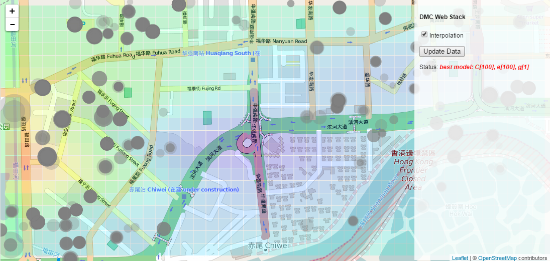
The final interpolation with cross-validation showing the parameters of the chosen best model
While it may seem tedious, this kind of iterative testing is a crucial component of Machine Learning. Since the setting of the model parameters are totally dependent to the data you have and the system you are trying to model, there is no way to know what these parameters should be from the start. The only way to determine the settings that will define the best model is to go through this system of cross-validation, and use a separate data set which has been set aside to evaluate and validate the models.
Testing your knowledge
This concludes our first example of Machine Learning for our Web Stack, using a supervised SVM model to interpolate housing prices across a study area. In the next set of tutorials we will explore other types of analysis, including further applications of Machine Learning. For now, switch to the 04-assignment branch in the ‘week-6’ repository. This branch contains the final version of the app.py file against which you can check your own work. To test your knowledge, try to implement the following features into the Web Stack:
- In the
index.htmlfile, create a user interface for switching between heat map and interpolation analysis. This can be a series of checkboxes, a drop down menu, or another type of form element - In the
index.htmlfile, create a user interface for setting analysis parameters such as the resolution of the grid, the ‘spread’ of the heat map, or the maximum number of data points that should be considered in the analysis - In the
script.jsfile, capture the options selected by the user in the client code, and pass them as arguments to the server within the request - In the
app.pyfile, capture the request arguments coming from the client in the server code and use them to control the parameters of the analysis
You will find helpful comments for implementing these features throughout the files in the 04-assignment branch. Remember to submit a pull request with your changes before the next deadline.