Putting it all together
In this tutorial we will combine all the basic features we have developed for our Web Stack so far. We will use D3 on the client side to request data from our Flask server, which will then query that data from the OrientDB database and return it to the client. Once the data is returned we will use D3 to visualize the data on a special overlay layer of the dynamic Leaflet map.
To start, switch to the 04-putting-it-all-together branch in the ‘week-3’ repository. Open up the app.py file in the main repository folder. This file has already been updated with a /GetData/ route which will query data based on a latitude/longitude bounding box from our database. Most of this code should be familiar to you, as it is the same basic query we developed in the Accessing OrientDB through Python tutorial.
The only major addition to the route function is how the results of the query are formatted before they are sent back to the client. Remember that the d3.json() function we are using to make the request on the client side is expecting us to return data in the JSON format. One advantage of using this format is that we can work with Python lists and dictionaries to define our own data structure, and convert it directly into a JSON format using Python’s json library. Another advantage, particularly in our case, is that we can directly utilize the GeoJSON format, which is a special implementation of JSON for geographic data that accounts for geometry types and attributes that are particular to geographic data. This format is useful because it can be used within other GIS software and can be converted to from other geo-data formats such as .shp. D3 also provides some useful functions for working with geographic data that we can tap into as long as our data is formatted in the proper way.
To format our queried results as GeoJSON data, we first create a main dictionary which will be stored in a variable called ‘output’.
output = {"type":"FeatureCollection","features":[]}
The first entry in this dictionary is a key/value pair that specifies the type of data we are storing, which in our case is a ‘FeatureCollection’. The next entry will store the feature data itself. It is referenced by the ‘features’ key, and the value is a blank list that we will fill with our feature data. Now we will fill this list by iterating over each record we received from the query, creating a feature record for it in the proper GeoJSON formatting, and appending it to the list of features.
for record in records:
	feature = {"type":"Feature","properties":{},"geometry":{"type":"Point"}}
	feature["id"] = record._rid
	feature["properties"]["name"] = record.title
	feature["properties"]["price"] = record.price
	feature["geometry"]["coordinates"] = [record.latitude, record.longitude]

	output["features"].append(feature)
We initialize each feature as a dictionary with some standard GeoJSON formatting. The first key/value pair specifies the type of object we are creating, which is a ‘Feature’. The next two key/value pairs create dictionaries which will store the ‘properties’ of the data point, which are all the non-geographic parts of the data, as well as the ‘geometry’, which specifies it’s geographic location. Within this ‘geometry’ dictionary we also add a key/value pair which specifies the type of geometry we are using, which in our case is ‘Point’. You can consult the GeoJSON Documentation for the various other kinds of geometry objects that are supported.
In the next few lines we will fill in the feature dictionary according to the data we receive from each record. We first create an ‘id’ key in the main dictionary which will store the unique ‘rid’ of the record in our database. Then we specify some of the non-geographic properties of the record. In this case we are only storing the ‘title’ and ‘price’ of the record since we would like to use this for visualization and processing later, but you can store any number of properties by simply adding them to the ‘properties’ dictionary. Finally, we add the latitude and longitude coordinates of the record to a new ‘coordinates’ key within the ‘geometry’ dictionary. After all the data has been specified, we append the new feature dictionary to the list of features within the main output dictionary.
The last line of our /getData/ function returns our new GeoJSON formatted dictionary as a json file by running it through the .dumps() function of Python’s json library.
return json.dumps(output)
Now that we have created a route on our server to return the geographic data, let’s develop some client code that will request the data and visualize it on our map. Open the index.html file in the /templates folder of the repository. This contains the basic Leaflet map code we developed in the last tutorial. We will write the rest of our client-side code within the same <script> tags following the Leaflet code. Much of this code was adapted from a good overview tutorial provided by Mike Bostock which covers basic integration between Leaflet and D3. Although some of the data implementation is different, you can consult this tutorial for more information about some of the D3 functionalities that are used.
Let’s start by creating some variables to store references to objects on the web page that D3 will draw the geometry to.
var svg = d3.select(map.getPanes().overlayPane).append("svg");
var g = svg.append("g").attr("class", "leaflet-zoom-hide");
The first line creates an empty ‘svg’ object that will contain all of our drawn geometry.
SVG, or Scalable Vector Graphics is a standard which is utilized by D3 for creating graphics on the web. SVG is useful because it can specify different kinds of basic geometry such as circles, rectangles, and lines in a format similar to HTML. This allows you to control their visual appearance through parameters directly within the website code, or through CSS styling just like you would with any web page element. To start working with SVG, you first create a main ‘svg’ object in the HTML code. You can think of this svg object as the ‘canvas’ on which you can draw geometry elements by appending them to the object. Within this main svg object it is useful to organize geometry elements within individual groups using ‘g’ objects, as we do here. Organizing geometry this way will allow you to reference different parts of the canvas, similar to how you would work with ‘layers’ in a vector graphics application such as Adobe Illustrator.
This svg object is appended to a special ‘overlayPane’ layer of the map created by Leaflet. Adding our geometry to this layer will ensure that it appears properly in front of any map elements. On the second line, we append a ‘g’ object to our new svg. The ‘g’ object represents a group that will contain all of our new geometry. We will also use the .attr() method to give the object a class of ‘leaflet-zoom-hide’, which will tell Leaflet to hide this object when the map is zoomed. This will create a better transition when the data is updated during a map redraw.
Next, we will create a function that will project points from their latitude and longitude geographic coordinates to x and y coordinates on the screen.
function projectPoint(lat, lng) {
	return map.latLngToLayerPoint(new L.LatLng(lat, lng));
}
This function utilizes Leaflet’s .LatLng() and .latLngToLayerPoint() functions to first create a point from lat/lng data, and then project it to the proper x/y screen coordinates relative to the current map view. You can consult the Leaflet documentation for more information about these two functions.
Next, we will write some code that will allow D3 to work with Leaflet’s projection system, and allow us to utilize some of D3’s helpful geometry functions for working with our GeoJSON data. Some of this functionality is quite advanced, so if you find it difficult to grasp don’t worry. You can utilize this code without completely understanding it, just know that it is a way for us to connect Leaflet, which is managing the map transformations, to D3, which will be working with the actual data and converting it to visualizations on the map.
function projectStream(lat, lng) {
	var point = projectPoint(lat,lng);
	this.stream.point(point.x, point.y);
}

var transform = d3.geo.transform({point: projectStream});
var path = d3.geo.path().projection(transform);
We first write a function that creates a geometry stream using the transformation function written previously. We then use this geometry stream to create a custom D3 transformation object which will be stored in a variable called ‘transform’. Finally, we use this transform to create a d3.geo.path() object that will be tied to the same projection system used by Leaflet to create our map. We can now use this new ‘path’ object to take advantage of some useful functions D3 has for processing geographic data, while ensuring that the geographic projection will always match our underlay map.
Now that we have established some helpful functions for transforming our geographic data, we will use the d3.json() function to actually request the data from our server, and then visualize it by drawing geometry to our map.
d3.json("/getData/", function(data) {

	var circles = g.selectAll("circle").data(data.features);

	circles.enter()
		.append("circle")
	    .attr("r", 10);

});
Into the d3.json() function we pass the request URL which matches the ‘/getData/’ route we set up on our Flask server. In the second argument (the ‘callback’), we write an anonymous function which will execute once the data is received and use the data to control the visualization. As long as we are in this anonymous function we will be able to reference the received data, so we will develop most of the rest of our code here.
Within the function, we first establish a variable called ‘circles’ to store a reference to our visualization geometry, which will use a circle to represent each data point. Within the ‘g’ object, we select all objects of type ‘circle’ using D3’s `.selectAll() method. Since there are no circles yet drawn, this selection will initially be empty. However, this selection will tell D3 where we want our geometry to be located within our web page’s structure. Once we have the selection, we ‘join’ it to the data we receive from the server with the .data() method. Into this method we pass the ‘features’ portion of the returned data, which contains our list of point features. This data ‘joining’ is a key feature of D3, which creates a direct connection between the geometric features in our selection to a collection of data.
This connection is super useful because it automatically calculates the correspondence between the geometry and the data, and creates new selections which allow us to update the visualization according to changing data. If there is less geometry than pieces of data (as in our current situation where no geometry has yet been drawn), we can use the .enter() selection to reference the data which has not yet been assigned. If there is more geometry than data, we can use the .exit() selection to reference the extra geometry. Joins can be difficult to grasp at first, but they are really the backbone of D3, and are the primary feature that make D3 such a useful tool for dynamic data visualization. For more background on data joins you should consult Mike Bostock’s tutorial here, as well as the extended discussion of D3’s update pattern.
Once the data join has been made, we reference the .enter() selection and use the .append() method to add a ‘circle’ geometry for every data point which does not have any geometry associated with it. We then use the .attr() function to set the ‘r’ attribute of the circle, which sets the radius of each new circle to a constant of 10 pixels. If you want to learn more about SVG, including the available geometry types and their parameters, you can consult this useful tutorial.
Next, we will create a function to update the location of the main SVG element, as well as each circle’s location within it according to the updated data. We do this within a function because we want the update code to run not only after the data is updated, but also any time the map is zoomed or redrawn, since this will also change the relative position of the SVG and the relative positions of the points on the screen.
function update() {
    var bounds = path.bounds(data),
        topLeft = bounds[0],
        bottomRight = bounds[1];

    var buffer = 50;

    svg .attr("width", bottomRight[0] - topLeft[0] + (buffer * 2))
        .attr("height", bottomRight[1] - topLeft[1] + (buffer * 2))
        .style("left", (topLeft[0] - buffer) + "px")
        .style("top", (topLeft[1] - buffer) + "px");

    g   .attr("transform", "translate(" + (-topLeft[0] + buffer) + "," + (-topLeft[1] + buffer) + ")");

    circles
    	.attr("cx", function(d) { return projectPoint(d.geometry.coordinates[0], d.geometry.coordinates[1]).x; })
    	.attr("cy", function(d) { return projectPoint(d.geometry.coordinates[0], d.geometry.coordinates[1]).y; });
};
Let’s break this function down line by line to see everything that is being updated. In order to update the size and location of the main SVG element, we first need to know the extents of the data relative to the screen. For this we use the .bounds() method of the path object we specified in the beginning of our code. Since this path object is tied to the same projection system used by Leaflet to draw the map, it can do useful things like getting the bounding box of all the data in screen coordinates. We store the bounding box coordinates in a variable called ‘bounds’ and create two more variables called ‘topLeft’ and ‘bottomRight’ to store the coordinates of the bounding box’s corners. We will now update the relative size and location of our ‘svg’ and ‘g’ objects according to this bounding box. However, since the bounding box will be related only to the center of the circles, we should add a buffer to make sure that none of the actual circles get cropped. To do so we create a ‘buffer’ variable which will store a buffer of 50 pixels.
Next, we use the ‘svg’ variable to change the properties of the svg canvas. We set it’s width and height to the current width and height of the bounding box, plus two times the buffer size. We also set it’s position to the top-left corner of the bounding box, minus the buffer. Since the location of the circles will be generated relative to the screen, but they will be drawn relative to the location of the svg, we should also offset the location of the ‘g’ element to correspond to the upper left hand corner of the screen. To do this we call the ‘g’ variable and update its ‘transform’ property to translate it the same amount as the svg but in the opposite direction. Now we can draw the points relative to their location on the screen and have them appear in the proper place, regardless of the limits of the svg canvas. You can consult Mike Bostock’s tutorial for a more in depth description of why these transformations are necessary.
Finally, we will update the location of the actual circle objects (stored in the ‘circles’ selection set). To do this we use the .attr() function of the circle objects to set their ‘cx’ and ‘cy’ position attributes. To set the actual position we use an anonymous function that updates the position of each circle relative to the data we have received. To convert the geographic coordinates stored in the data to screen coordinates, we will use the projectPoint() function we established earlier in our code.
After our update function has been defined, we will call it once to make sure that the graphics are updated when data is received. We will also use the map object’s event handling method .on() to tell it to run the update() function every time the map experiences a ‘viewreset’ event, which will happen any time the map is redrawn (this happens on page load and zoom, but not in simple panning).
update();
map.on("viewreset", update);
In addition to controlling the properties of SVG elements through D3’s .attr() method, you can also control global properties of SVG elements through CSS, just as you would for any HTML element. In the <head> portion of the document, add another property within the <style> </style> tags:
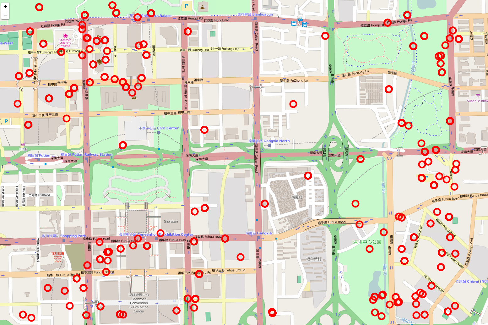
circle {
	fill-opacity: 0;
	stroke: red;
	stroke-width: 5px;
}
This will set some global style parameters to all ‘circle’ elements on the page. Here we set the fill to transparent, change the stroke (another word for outline) color to red, and the thickness of the stroke to 5 pixels. For more examples of SVG styling and the available parameters you can consult this SVG tutorial.
Congratulations, our basic implementation of the Web Stack is complete! Using this basic structure we can develop different user interaction features that can create requests for data from the server, and visualize this data back to the user. We will build on this framework to develop various UI and data processing function in the rest of the tutorials. If you are having issues getting any of the code to run, switch to the ‘05-assignment’ branch in the ‘week-3’ repository to see what the final code should look like. Then, test your knowledge by completing the instructions in the index.html file to implement dynamic sizing of the circles according to price data. You can also experiment with further styling of the svg elements by adding your own CSS styling rules to the <head> of the document. Remember to submit a pull request with your changes before the next deadline.